
Time series data is a collection of data points recorded over time, that are used to analyse trends and patterns in a specific variable. This type of data is commonly used to track financial indicators, weather conditions, and website metrics. Forecasting time series data is an important task that can be achieved using various methods. Two naive approaches are to use the last observation or the average of all past observations as the basis for future predictions. A more sophisticated approach is to combine these two strategies using exponential smoothing.
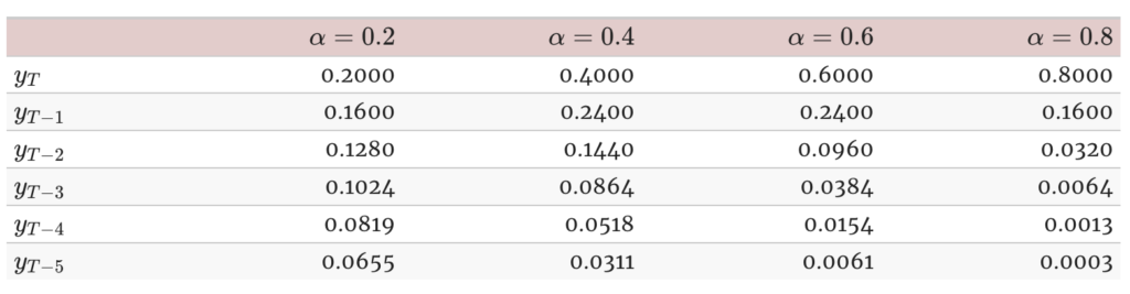
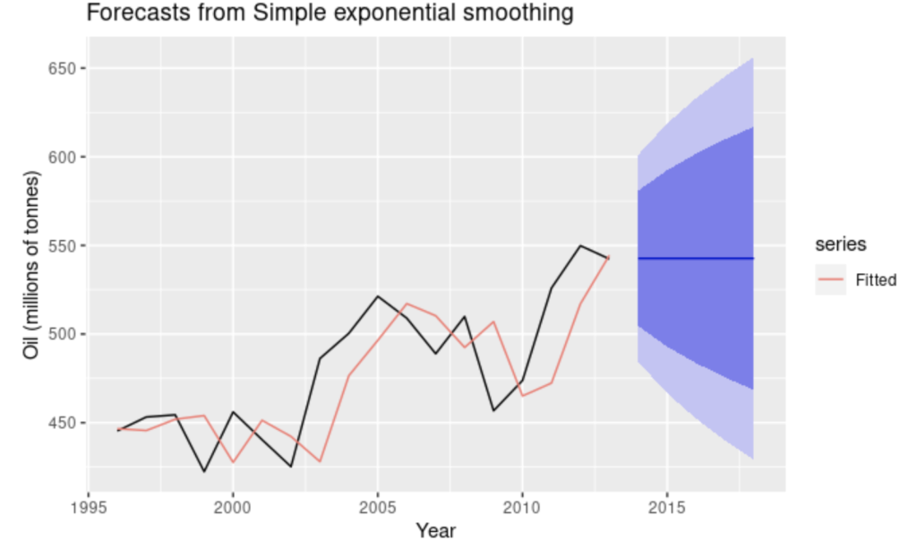
Simple exponential smoothing is a weighted average method that assigns larger weights to more recent observations and smaller weights to older observations. The weights decrease exponentially as the observations get further from the present. The choice of smoothing weight, or α, is an important decision that can significantly impact the accuracy of the forecast. A higher smoothing weight gives more weight to the most recent observations. On the other hand, a lower smoothing weight gives more weight to past observations, and has a greater smoothing effect.
While simple exponential smoothing is a good starting point for forecasting time series, it does have limitations. The main drawback is that it assumes no trend or seasonality. If there is a trend in the data, such as a gradual increase over time, simple exponential smoothing will not capture it. Similarly, if there is seasonality in the data, such as a monthly pattern, simple exponential smoothing will not account for it.
Holt-Winters Exponential Smoothing
To capture trend and seasonality, the Holt-Winters (also known as ETS; error, trend, season) method can be used. This method extends simple exponential smoothing by adding a trend and seasonal component to the model. The trend component captures the direction and magnitude of any overall trend in the data. The seasonal component captures any seasonal patterns that repeat over a fixed period of time.
In some cases, it may be useful to incorporate a damping effect in the trend, as the trend has a tendency to be over exaggerated. This can be accomplished by introducing a parameter into the trend equation, which is a constant value that controls the damping. This results in a trend that gradually approaches a steady state, rather than continuing to increase or decrease indefinitely
The seasonal component is calculated by averaging the values of the same season across all years in the time series, with a weighted average. For example, if the time series has monthly data, the expected seasonal value for January would be the weighted average of all January values in the time series.
The final equation is as follows:
Forecast t+1 = Level t + Trend t + Season t
Where level, trend and season are all based on the weighted average of past values.
Parameter selection
The three elements can be combined either by addition or multiplication.
Additive combination is used when the amplitude of the seasonal pattern does not depend on the level or trend of the time series. It is best suited for data where the seasonal fluctuations are relatively constant over time. In this case, the seasonal component is simply added to the equation to produce the forecast.
Multiplicative combination is used when the amplitude of the seasonal pattern varies with the level of the time series. This is best suited for data where the seasonal fluctuations increase or decrease proportionally with the level of the time series. In this case, the seasonal component is multiplied by the level of the time series to produce the forecast.
This means there are ways to combine the three components together, represented using a three letter abbreviation. For example ETS(A,Ad,M) would mean an Additive error, Additive damped trend and Multiplicative season. One point to watch out for, is that depending on the data some of these models can be unstable. As an example, if the data contain 0’s or negative values, then multiplication can cause errors.
Model selection
We have many potential combinations of parameters and smoothing coefficients. Fortunately, most programs will automatically try many different combinations. However we still need a way to select the best model. It would be a mistake to use something such as R2 , as that could lead to overfitting. Instead a measure known as an information criterion is used, which is a statistical method for evaluating a model’s performance.
Implementation
ETS can be directly implemented using a programming language such as python. Alternatively, a no-code tool with this functionality, such as Alteryx could be used. This allows you to implement a forecast with just a few clicks. Here is what a barebones implementation in Alteryx looks like.
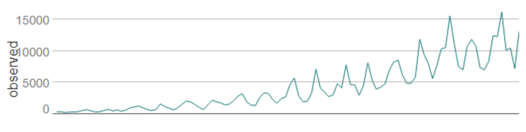
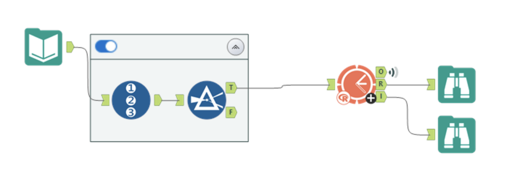
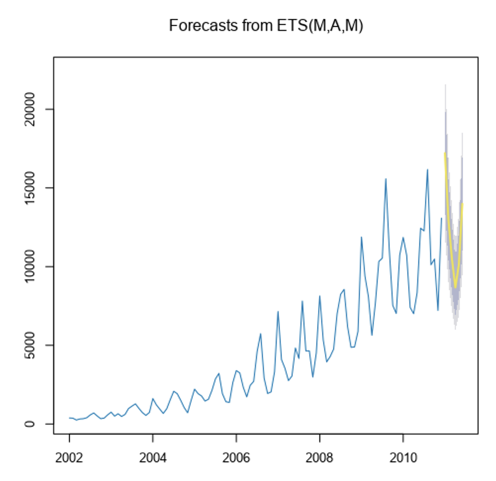
We can see that our forecast has successfully captured the trend and seasonality of our data. In this case we use a multiplicative model, because the seasonal swings grow in size as the trend increases.
Conclusion
Exponential smoothing is a tried and tested technique for forecasting time series data. When used correctly it can produce accurate forecasts that take the seasonality and trend of your data into account. To learn more, Forecasting principles and Practice is a good starting place. The authors provide a clear overview of important fundamentals without going into the weeds. To learn more about visualizing time series data, check this post out.
Have Fun!