In a previous blog post, we delved into the world of time series forecasting with the Holt-Winters (exponential smoothing) model. Today, we will explore another popular forecasting technique: the ARIMA model.
ARIMA, which stands for Autoregressive (AR) Integrated (I) Moving Average (MA), is a statistical model that combines three different components to make a forecast. Let’s start with the I component.
Integration
Stationarity refers to the consistency of a time series’ statistical properties over time. In a stationary time series, features such as trends and seasonality do not affect the data’s value at different times. For example, a white noise series, which looks similar at any point in time, is considered stationary. In general, a stationary time series exhibits no long-term predictable patterns. When plotted, it appears roughly horizontal, maintaining a constant variance, though some cyclic behavior might still be present.
The ARIMA model is designed to work with stationary data. We achieve this by employing a technique called differencing. Differencing involves calculating the difference between each data point and the previous one, which eliminates trends or seasonal patterns. By applying differencing, the original non-stationary data can be transformed into a stationary form, which is required for forecasting with the ARIMA model.
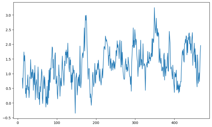
This time series is clearly not stationary
The term “integration” in the ARIMA model refers to this process.It is denoted as I(d) where ‘d’ represents the number of times it has been differenced. When it is differenced once, it is denoted as I(1). If it is differenced again, it is integrated of order two, or I(2), and so on. This is repeated until it is stationary. In the first figure, the series is not stationary. The second figure shows the same series that has been differenced once and appears mostly stationary.
The time series has been differenced once (Note that in this case, we have differenced it with a value 12 periods prior, due to the seasonal nature of the data which repeats every 12 steps)
The Auto Regressive Component
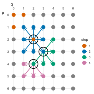
The AR component is simply a forecast of a future value based on a linear combination of previous values. It is often denoted as AR(p), where ‘p’ represents the number of past observations taken into account when modeling the current value. For example, an AR(1) model would use the value of the immediately preceding observation, while an AR(2) model would consider the values of the last two observations as follows;
The MA component is denoted as MA(q), where ‘q’ represents the number of past error terms considered when modeling the current value. The error terms represent the differences between the actual values and the values predicted by the AR component. You can think of the MA component as an error correction for the AR component.
Tuning the model
At this point we are ready to make our forecast. We need to decide on values for AR(p), I(d) and MA(q). I(d) is usually something you can decide on yourself – you need to make your data stationary. An algorithm is normally used to select the best values of p and q. The algorithm uses a metric (an information criteria or MLE) to determine the best parameters for the model.
https://otexts.com/fpp3/arima-r.html
Seasonal Data
Seasonal ARIMA, often denoted as SARIMA, is an extension of the ARIMA model designed to handle time series data with seasonal patterns. While the ARIMA model effectively captures trends and relationships in non-seasonal data, It does not work with seasonal data. SARIMA goes a step further by explicitly accounting for seasonality. This enhanced model incorporates additional parameters for seasonal autoregressive, seasonal differencing, and seasonal moving average components, allowing you to make forecasts with seasonal data
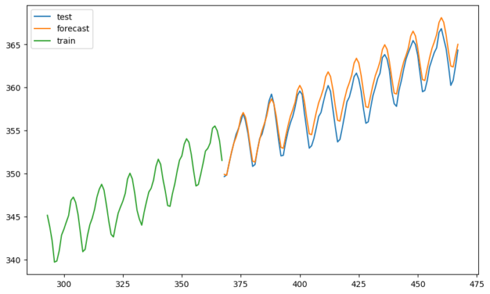
Our original time series, with an accompanying forecast. The model has captured the seasonal component.
Conclusion
The ARIMA model is a powerful and versatile tool for time series forecasting. By addressing the issue of stationarity through differencing and capturing the relationships between past observations and errors, the ARIMA model can make accurate and reliable predictions. Determining the optimal values is an essential step in the forecasting process, often achieved through the use of algorithms and information criteria. With a strong understanding of the ARIMA model’s components and assumptions, you can better understand its limitations and strengths.